WSPR 40M Propagation Explainer by Jim Willis

At one time low frequency (below 550 kHz) beacons were used for radio navigation in ships and airplanes. I imagined driving around listening for my beacon and doing direction finding or propagation experiments. That thought lasted about a minute, but I still wanted a beacon. And then along comes WSPR. Wow, now I can have my very own beacon! I ordered the excellent WSPR Desktop Transmitter from Zactech[1], outputting about 250 [mW], into an end fed half wave antenna. A month later I had some surprising experimental results. This paper attempts to explain those results.
Figure 1 - The excellent WSPR transmitter beacon from ZachTek. The beacon was programmed to transmit every ten minutes on 40 meters.
Available from: https://www.zachtek.com/product-page/wspr-desktop-transmitter
The WSPR Network
WSPR is a network of receivers connected by the internet to a central database. When a receiver decodes the message from a WSPR transmitter, it relays the information to the database. The message consists of the transmitting station’s callsign and QTH, the frequency, the receiving station’s callsign and QTH, the date and time and signal to noise ratio. I’m going to call the date/time and distance a “spot”.
Figure 2 - Station N5SNT, San Antonio, Texas received station KX4TD at 08:52 Zulu on 4/4/2020 at a distance of 1454 kilometers.
Figure 3 - A day's worth of spots. The example shown is the same as in Figure 2.
The plot of distance versus date/time for a day’s worth of spots surprised me! I expected to see the band fade in and out during the day. I was surprised at how the band has these regions of propagation and no propagation. There is some fading going on but mainly the band changes due to cutoffs in the “skip” and maximum propagation distances. It is not like a volume control knob; it is more like a sharp cutoff switch.
Looking at just the spots, shown in Figure 4, during the daytime (around local noon), the band extends from about 500 [km] to about 1500 [km]. During the night time in Figure 5, the band extends from about 1500 [km] to about 3500 [km]. During the “greyline” (dusk and dawn) the band extends from 0 [km] to 3500 [km]. I’ll explain what I think is happening during these three periods.
Figure 4 - There is an interesting pattern here. The band goes "long" during the night and “short” during the day.
Figure 5 - During the nighttime, the band extends from about 1500 [km] to about 3500 [km].


Radiation from the sun causes ionized layers to appear in the ionosphere. During the daytime (direct sunlight) there is a layer called the E-layer. During the nighttime, the E-layer disappears, and we are left with the F-layer. The E-layer is at a much lower altitude and cuts off signals to the F-layer. The F-layer is present day and night, but its strength diminishes during the night. Let’s look at nighttime propagation on 40 meters. For complicated reasons, only a small sliver of the F-layer can reflect 7 MHz radio signals. This means nighttime propagation on 40 meters goes from about 1500 [km] to about 3500 [km], as shown in Figure 6.
Figure 6 - During the nighttime, propagation is due to the F-layer, at an altitude of about 450 [km]. The result is propagation from about 1500 [km] to about 3500 [km].

During the daytime, the E-layer appears underneath the F-layer, as shown in Figure 8. The E-layer is at a much lower altitude and is more strongly ionized than the F-layer. This means a wider slice of the ionosphere supports propagation on 40 meters and because of the lower altitude, the propagation distances are shorter than at night. Which brings us to the greyline (dawn and dusk). Greyline is the period when F-layer is strongest and the E-layer fades away. Sometimes this allows near vertical incidence skywave (NVIS) propagation bringing the skip distance down to zero. This allows propagation from 0 [km] to 3500 [km]. The azimuthal map, centered on my QTH and shown in Figure 11, shows propagation distances for the three periods, nighttime, daytime and dusk. Greyline includes all three. Of course, with all these changes in the E and F-layers, the number of contacts made must also go up and down during the day. For example, consider a vertical slice one hour wide on Figure 9. If you count the number of spots during each hour, you come up with a graph shown in Figure 12.
Figure 7 - During the daytime, the band extends from about 500 [km] to about 1500 [km].
Figure 8 - During the daytime, propagation is due to the E-layer, at an altitude of about 60 [km]. The result is propagation from about 500 [km] to about 1500 [km].
Figure 9 - During greyline (dawn and dusk), the band extends from about 0 [km] to about 3500 [km].
Figure 10 - During the greyline, propagation is due to the F-layer. The result is propagation from about 0 [km] to about 3500 [km].


Figure 11 - Azimuthal map showing the propagation on 40 during the daytime, nighttime and dusk. At dusk, propagation extends from 0 [km] to 3500 [km].
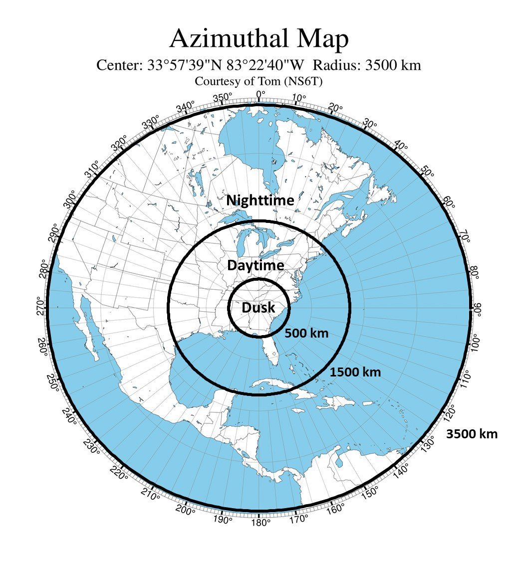
Figure 12 - The number of spots per hour changes throughout the day by a factor of four. If you were operating at 0100 Z you'd think the bands were hopping, at 1700 Z not so much.

Bonus and Limitations
So far we’ve looked at one day of spots and between 0 [km] and 4000 [km]. I’ve actually received spots all the way out to 20000 [km]! What’s happening here? We have only considered one-hop propagation. What happens with two hop propagation? The pattern repeats but only during the nighttime when the E-layer is not present. Referring to Figure 13, notice the gaps between 3500 [km] and 5000 [km]. Between 5000 [km] and about 6000 [km] and between about 8000 [km] and 13000 [km]. What’s going on here. Then I noticed the diagonal line shown by the arrow. What? A moving island? Well, sorta. It was a research vessel on its way to Antarctica. How’d I know this? His callsign and a lookup on QRZ. This points out a limitation in the WSPR technique; the limitation of the number of receiving stations. Some of these gaps in the spot plot are simply due to the absence of receivers. We are currently at the bottom of the sunspot cycle. These results will change as conditions improve. Thanks for reading this report and enjoy the hobby.
Figure 13 - Here is a plot of one month's worth of spots. Notice the steady progression of spots just above the arrow. What is going on?

Want even more on WSPR from Jim Willis KX4TD, well you are in luck. Click the image below and you'll see a video from W5KUB!
